Overall approach¶

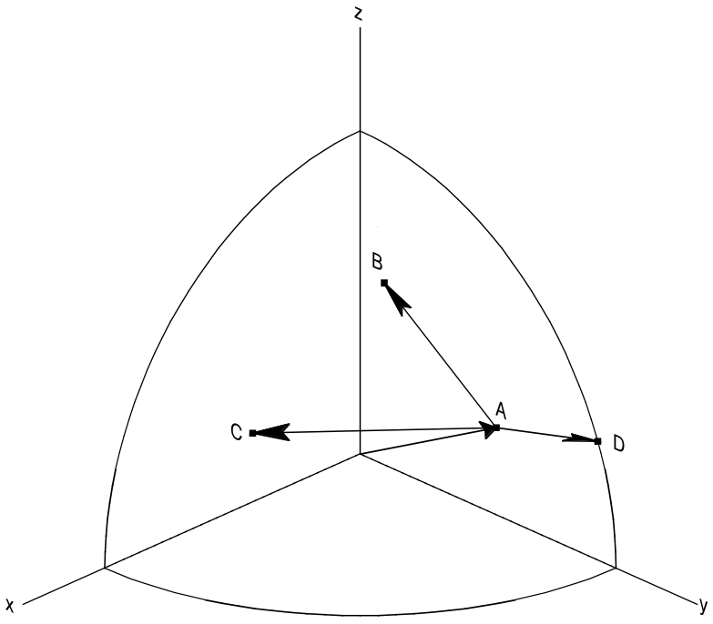
Figure 1 Illustration of an example pinwheel pattern that is searched for in the reference objects. Points A, B, C, and D are source points ordered from brightest to faintest. To find a match all lengths of the pinwheel spokes (e.g. \(|v_B - v_A|\)) and opening angles between spokes (e.g. the angle between vectors \(v_B - v_A\) and \(v_C - v_A\)) must be within tolerances \(\delta_{tol}\) and \(\delta_{ang}\) respectively. Shifts and rotations between the source and reference catalog are tested against the unit vector \(v_A\) and vector delta \(v_B - v_A\) respectively.

Both OPMb and PPMb construct “pinwheel” shapes that are used to search within the reference objects from the detected source catalog by ordering the objects in the catalog from brightest to faintest flux. The image in Figure 1 shows this pinwheel in three dimensions. The pinwheel is created by choosing the first first \(N\) brightest objects, treating the brightest of these as the pinwheel center (labeled \(A\)). The fainter If this pattern is not found in the astromtetric references then the brightest source is discarded and a new \(N\) point pinwheel is constructed starting with the second brightest object and so on until a requested number of patterns have been tested. In the current LSST implementation, the default value of \(N\) is 150.

Initialization¶

The PPMb algorithm begins by creating the data structures needed to both search for individual pattern spokes based on their distance and to compare the opening angle between different spokes. For each reference pair we pre-compute the 3-vector delta (\(v_{\Delta}=v_B - v_A\)), distance between the objects (\(|v_A - v_B|\)), and catalog IDs of the objects that make up the pair. Each of these arrays is sorted by the distance. We also create a lookup table that enables quick access to all pairs featuring a given reference object.

Shift and rotation tests¶

After selecting \(N\) sources ordered from brightest we compute the \(v_{\Delta}\) of the first two brightest points, and search for reference pairs with a distance \(|v_R|\) that have the same length to within \(\pm \delta_{tol}\) of the length of the source vector \(|v_S|\). We test each of these reference pairs from the smallest length difference \(\Delta = abs(|v_S| - |v_R|)\) to the largest, assuming that the correct pattern has nearly the same length for the source and length deltas.

These candidate pairs are then tested by first selecting one of the two reference points that make up the pair as the center of the pinwheel. By taking the dot product of the two unit-vectors representing the source center and candidate reference center, we can quickly check if the implied pointing shift is within the maximum allowed. If the shift is too large we then check against the other point in the reference pair. If both fail then we move to the reference pair with the next smallest \(\Delta\) and repeat.

Once a candidate reference pair and reference center are found to within the distance and shift tolerance, we compute the rotation matrix to align the source and reference centers. We apply this rotation to the source 3-vector rotating it into the reference frame. We then compute the dot-product of this 3-vector with the candidate reference 3-vector delta to compute the implied rotation of this candidate pair. If it is greater than our set maximum we continue to the next candidate reference pair.

Pattern construction¶

Assuming the reference candidate for the two brightest objects in the source pinwheel satisfies all of the previous tests we begin to create the remaining spokes of our \(N\) point pinwheel, in order of decreasing brightness. We first pare down the number of reference pairs we need to search by using the ID lookup table to select only reference pairs that contain our candidate reference center. This speeds up the next stages of the search significantly. We search for the reference spokes that match within tolerance in the same way as the previous step.

Once we have the candidates for this source spoke we need only test that the opening angle between this spoke and the initial spoke are within tolerance to the angle formed by the candidate reference objects. We make the assumption here that the separations between any point in the source or reference objects are small enough that we can assume simple 2D relations and that our dot and cross-products of difference vectors are within the plan of the sky.

We employ two separate but related tests to check that the opening angle between source pattern spoke we are testing and the spoke created by the two brightest source objects in the pattern is within tolerance of the corresponding reference angle.

We start by establishing the appropriate tolerance, \(\delta_{ang}\). Given the \(L\), the length of the source spoke being tested, we define:

This sets tolerance allowed between the reference and source pattens when comparing opening angle between two spokes. This avoids the user having to specify an arbitrary tolerance when configuring the algorithm. We set a limit that this angle be less than \(0.0447\) radians. This is set such that \(\cos(\delta_{ang}) \sim 1\) to within 0.1%. This allows us to use the small angle sine and cosine expansions in the coming comparisons. The tolerance assumes that \(L \gg \delta_{tol}\). When this is not the case, we instead set the opening angle tolerance to the value \(0.0447\). One can see examples of the angle under test in Figure 1 as the opening angle between the vectors \(v_B - v_A\) and \(v_C - v_A\): we ensure tha that the angles between these vectors as measured in the source and candidate reference patterns differ by no more than \(delta_{angle}\).

To test the opening angle against the current tolerance for this spoke, we compute the normalized dot-product between our source spoke to the first source spoke and do the same with the candidate reference spokes. We then test the difference of these two cosines:

If we assume that at most \(\theta_{src} = \theta_{ref} \pm \delta_{ang}\) and Taylor expand for small \(\delta_{ang}\) then we can write our test as

To avoid an expensive calculation of \(\sin\theta_{ref},\) square the above, giving:

This test on the difference in cosines is insufficient to demonstrate that the two opening angles are the same within tolerance because it does not test chirality and because of degeneracies due to the periodic nature of the functions.

To completely test that the angles are within tolerance we also need to test the sine of the angles. Here, we compute the normalized cross-product between the two source spokes and likewise the reference spokes. This produces vectors with lengths \(\sin(\theta_{src})\) and \(\sin(\theta_{ref})\) respectively. These vectors can be dotted into the center point of the the respective patterns they are derived from giving the value of the sine. It should be noted here that the value is approximate as the vectors are likely slightly misaligned to that of center points, artificially decreasing the amplitude of the sine. However, on the scale of a a CCD, the vectors we are comparing are within the plane of the sky and thus the comparison holds.

If we again Taylor expand for small angle differences the comparison becomes

These tests in tandem assure us the opening angles are the same between the source and reference spokes and that they rotate in the same direction. The tests are robust for all values the opening angles for both the reference and source patterns.

Intermediate verification¶

Once we have constructed the complete pinwheel pattern of the requested complexity, we test that the shift and rotation implied by the first spoke in each of the source and reference pinwheels can align the reference and source patterns on top of each other such that the distances between the source and reference points that make up the pinwheels are all within the matching tolerance. If this condition is satisfied we then fit a rotation matrix using the \(N\) matched points that transforms source objects into the reference frame. To permit for some distortion in the final verification process, this matrix is allowed to be non-unitary.

Pessimism of the algorithm¶

Up until this point PPMb has followed roughly the same algorithm as OPMb, although it uses vectors in 3-space on the unit-sphere instead of on the a focal plane. However, having successfully completed intermediate verification, the approaches diverge.

A series of test points are generated by computing the mean 3-vector of the source sample and creating six points by replacing each Cartesian coordinate in turn first by the minimum and then the maximum of the sample (thus \([x_{min}, \overline{y}, \overline{z}]\), \([y_{max}, \overline{y}, \overline{z}]\), etc).

Upon finding a candidate reference pattern we rotate the test points from the source into the reference frame using the rotation produced by intermediate verification. We then store these rotated test points and continue our search, starting another \(N\) point source pinwheel pattern. Once we find more patterns that pass intermediate verification, we rotate the 6 points again and compare their rotated positions to previous shifts and rotations that have been matched. If a user-specified number of previous shifts and rotations move the test points to within the \(\delta_{tol}\) length tolerance then we can proceed to the final verify step.

In tests we have shown that finding three such matches reduces the false positive rate for dense stellar fields significantly even for large values of \(\delta\). We also set a threshold for using this pessimistic mode requiring that both the number of reference objects and source objects exceeds the total number of source patterns to test before softening tolerances. This assures us that there are enough objects to have the desired number of matching patterns.

Final verification¶

Finally, after finding a suitable shift and rotation matrix we apply it and its inverse to the source object and reference object positions respectively. We construct searchable k-d trees using the spatial algorithm in SciPy. This is done for both the source and reference objects in their respective frames for fast nearest-neighbor look up. After matching the rotated source and rotated reference objects with the k-d tree we construct a “handshake” match. This matching refers to having both the sources matched into the reference frame and the reference matched into the source frame agree on the match in order to consider it valid. This cuts down on false positives in dense fields. After trimming the matched source and references to the maximum match distance \(\delta_{tol}\), we test that the number of remaining matches is greater than the minimum specified. Once this criteria is satisfied we return the matched source and reference catalog.

Softening tolerances¶

PPMb has two main tolerances which can be softened as subsequent attempts are made to match the source data to the reference catalog. These are the maximum match distance \(\delta_{tol}\) and the number of spokes which can fail to find a proper match before moving on to the next center point. We soften the match distance by doubling it after the number of source patterns requested has failed. We also independently add 1 to the number of spokes we attempt to test before exiting. We still require the same \(N\) point complexity of the pattern but we can test a total number of \(N-M-2\) spokes before exiting. These two softenings allow the algorithm enough flexibility to match to most stellar densities, cameras, and filters.

Fraction of successful matches¶

In this section we compare the rate at which PPMb and OPMb are able to find acceptable matches on datasets spanning different densities of objects, data quality, and bandpass filters. For each dataset we set an upper-limit on what we consider a successful match/fit cycle based on the expected quality of the astrometric solution after a successful match. This are 0.02 for New Horizons and 0.10 for both CFHTLS and HitS. These numbers were derived from confirming successful matches by eye and noting the RMS scatter in arcseconds of the final astrometric solution.

In the results tables below:

• “N Successful” is the number of CCDs where a match has been found;
• “N Failed” is the number of CCDs where a match was not found;
• “Success rate” is the ration of “N Successful” to the total number of CCDs.

Match quality comparisons¶

In addition to the looking at the fraction of successfully matched CCDs, we also examine at the quality of those matches and the astrometric solutions they produce

First we present the results for all CCDs that were successfully matched and solved by the two algorithms. For the New Horizons sample, we see that the solutions produced by OPMb are of poor quality: their RMS scatter on the solution is greater than several times the pixel scale (\(\sim 0.16\) arcseconds). PPMb fares better, although some solutions still have a large RMS scatter and pull both the mean and variance to higher values.

For HiTS and CFHTLS the two algorithms are more comparable with PPMb having a slightly wider distribution around the average solution.

The following table shows the summary statistics computed on the same data as above but now \(5 \sigma\) clipped around the mean to compare the results with outliers removed.

Run-time tests¶

One concern with the generalizations added to OPMb to make PPMb is if the algorithm can still find matches in running time comparable to that of the current Stack implementation of OPMb. In this section we present timing results both for a field with low density and with a high density. We count the time spent matching from the moment the doMatches is called until an array of matches (even if it is empty) is returned. We run through all CCDs in the CFHTLS in the g, r sample run previously and all of the CCD-exposures in NH pointing 908. For both methods there are outliers that heavily skew the mean and variance and thus we clip the times with a \(5 \sigma\) iterative clipping.

Both the mean and the median figures above suggest that PPMb is between 10% and 30% slower than OPMb for these datasets. However, it should be noted that PPMb is currently implemented in pure Python using NumPy. The main pattern creation loop of PPMb relies mostly on internal Python iteration which can be very slow. This is in comparison the Stack implementation of OPMb which is coded in C++. The extra steps of PPMb then do not catastrophically increase the compute time to find astrometric matches.